
Forecasting a Trial Before It Finishes
A Bayesian joint model that reads tumour scans as survival evidence
2026-07-30
We have a new paper out: PIONEER: Bayesian Joint Modelling of Mechanistic Tumour Growth and Time-to-Event Endpoints for Dynamic Prediction of Ongoing Oncology Trials. This post is the plain-language version — what the model is, what we ran it on, and what it did.
The decision you cannot postpone
Somewhere around the middle of a Phase 2 oncology trial, a team has to decide whether to keep going. The difficulty is structural. Progression-free survival and overall survival are the endpoints the decision rests on, and both are measured by how long patients go without progressing or dying — so at an interim look, most patients’ outcomes are simply still unfolding. A patient with nothing recorded yet is not a patient known to be doing well; they are someone we have not been following long enough to say. The median of anything is a long way off, and the primary endpoint may not read out for another year or more.
Waiting is not free, and neither is guessing. So teams reach for whatever will carry the weight — a p-value on immature data, a comparison against a historical control, an assumed effect size and a conditional-power calculation. Each of these is a way of not-quite-answering the actual question, which is: what will this trial look like when it finishes?
The evidence already in hand
Here is the thing that motivated the paper. At every interim cut-off, that trial is sitting on a dense, information-rich record that a survival analysis almost entirely discards.
Patients get scanned on a schedule. Each scan yields a sum of longest diameters — a number for how much tumour is present. Over months, each patient accumulates a trajectory. A conventional interim analysis compresses all of that into a single fact: “progressed at week 14”, or “not yet progressed”. Six measurements tracing a tumour shrinking, bottoming out, and starting to regrow become one event indicator and one date.
But the shape of that trajectory is exactly what tells you where a patient is heading. A tumour still shrinking at last contact and one that bottomed out three months ago and has been climbing since are in very different positions — and a survival model that sees only “no event yet” treats them identically.
The model, in three pieces
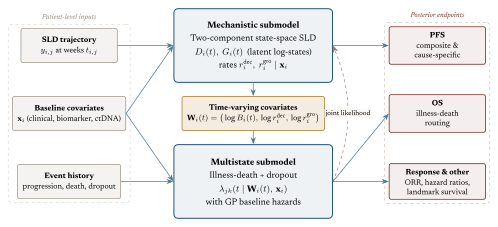
The framework couples three components and — this is the load-bearing part — fits them simultaneously, under a single posterior.
Tumour dynamics. A mechanistic state-space submodel infers each patient’s latent tumour trajectory from their sparse, noisy scan measurements. It is a two-component decomposition: tumour burden is split into a treatment-responsive compartment that shrinks under therapy and a refractory compartment that does not, with Gompertz-attenuated growth so that regrowth decelerates as burden accumulates rather than running away exponentially. The familiar shrink-then-regrow curve falls out of the two compartments crossing over — it is not imposed.
Clinical events. A multistate proportional-hazard submodel handles the events that actually happen to patients — progression, death with and without prior progression, dropout — as transitions between states rather than as a single lumped endpoint. The latent tumour trajectories enter this submodel as time-varying covariates. The hazard responds to where a patient’s tumour is going, not merely to their baseline risk factors.
One joint fit. The arrow runs both ways. Latent trajectories drive the hazards, and the event data simultaneously sharpens the tumour dynamics through the shared likelihood. A patient who progresses tells the model something about their tumour trajectory, not just the other way round.
That bidirectionality is what distinguishes this from the standard two-stage pharmacometric workflow, where you fit tumour kinetics first, extract summary statistics — growth rate, time to nadir, week-8 burden — and plug them into a survival model as though they were measured without error. Two-stage inheritance discards the uncertainty in stage one and attenuates the association in stage two. Fitting jointly avoids both, at the cost of a considerably harder posterior.
Every endpoint — PFS, OS, objective response rate — is then derived from that single joint posterior in one forward simulation pass. Not three models reconciled after the fact; one model, simulated forward, with full parameter uncertainty carried through.
The data
The case study is first-line extensive-stage small-cell lung cancer, using two completed trials obtained through Project Data Sphere — public, checkable data rather than a private case study nobody can audit.
| Trial | Role | N | |
|---|---|---|---|
| Target | Lilly CXCR4 (I2V-MC-CXAC) | the trial being forecast | 78 |
| Historical | Amgen 20010145 (darbepoetin alfa) | the trial borrowed from | 419 |
The design is a retrospective replay. Both trials are finished, so we know the answer. The model is re-fit at successive historical cut-offs, given only the data that existed at that moment, and its forecast is compared against the mature result it had not yet seen. This is leave-future-out cross-validation, and adapting it to this setting is fiddly enough that I wrote a separate post about it.
The 419 historical patients matter because nine patients cannot determine a survival curve on their own — but they do not have to. Growth kinetics are partially pooled across both trials, with the degree of borrowing learned from the data rather than fixed in advance. The target trial’s own patients still decide the final answer; the historical trial supplies the shape of the process.
Does it work?
Start one level below the survival curves, at the thing the mechanistic submodel actually produces: a trajectory for each individual patient, continued past the point where their data stops.

This is the step that makes the rest possible. Each of these patients is censored — no progression recorded — so a conventional analysis has nothing to say about them beyond “still enrolled”. The model instead carries each one forward with an explicit uncertainty band, and those simulated trajectories are what drive the hazard, which is what produces the survival curve below.
Now the retrospective replay for progression-free survival. Each column is a cut-off, labelled with how many target-trial patients had enrolled by then.

At month 4, with nine patients enrolled, the 80% credible band already covers the mature Kaplan-Meier curve — the dashed line the model had not yet seen, and would not see for another fifteen months. The band is also very wide — which is the correct width for what nine patients can support.
By month 11, at 39 patients, the forecast has tightened onto the mature curve. Tracking the median directly makes the convergence easier to read:


Overall survival converges at month 11 — at least eight months before it actually read out, with uncertainty properly quantified rather than asserted. The OS intervals are wider than the PFS ones throughout, and they should be: OS routes through progression, direct death, and dropout, and the forecast carries all three.
What this does and does not show
Coverage is not the same thing as a decision.
That the month-4 band contains the truth says the model was not wrong. It does not say the model was useful at month 4 — a band that wide is consistent with several conclusions at once. What a decision needs is an interval narrow enough to separate “keep going” from “stop”, and at month 4 this one is not. Read properly, month 4 says wait.
This is worth stating as a property rather than an accident: when the model cannot forecast well, that shows up in the output rather than hiding behind it. Uncertainty about the tumour parameters, about the hazards, and about where each unfinished trajectory is heading is carried through the same posterior into the endpoint, so sparse or uninformative data produces a wide band. The month-4 panel is the model reporting that nine patients do not determine a survival curve. There is no separate diagnostic to consult and no quiet failure mode where a confident-looking number comes out of data that cannot support it — the width is the diagnostic, and it is in the same picture as the answer.1
The value is not one heroic early number. It is knowing, at every cut-off, which conclusions the data currently support and which it does not — and being told that on the endpoint’s own scale, in months of survival, rather than as a single probability of success.
That distinction is worth being precise about, because the usual interim tools differ from each other. Conditional power gives the chance of a significant result at the final analysis given an assumed treatment effect — and that assumption then becomes the thing under debate, since the answer moves with it. Bayesian predictive probability of success is better on exactly this point: it integrates over the posterior for the effect instead of fixing it. But both collapse the picture to one number relative to a pre-specified success threshold. Forecasting the mature curve keeps the estimate and the threshold apart: the model says where the endpoint is heading and how uncertain that is, and where the go/no-go line sits stays an explicit statement of risk tolerance — the stakeholder’s to make, not the model’s.
I would also flag the obvious limitation: this is one indication, two trials, one retrospective replay. It is evidence that the approach works, not evidence about how well it works in general. Extensive-stage SCLC is a fast-moving disease with a strong tumour-burden signal, which is a comparatively favourable setting.
The natural next question is whether it holds up elsewhere, and a second application — a different disease, a different set of trials — is in progress. Results will follow in a later post.
Where to go next
The paper has the full specification — the state-space formulation, the multistate hazard structure, the hierarchical priors, and the cross-validation methodology. If you want the cross-validation piece on its own, the LFO post works through what breaks when you take a method built for univariate time series into a setting with staggered enrolment and two different observation clocks.
If you are working on something structurally similar — a latent mechanistic process generating both a longitudinal measurement stream and an event stream, with actors entering at different times — I would be glad to hear about it. The skeleton is not specific to oncology.
Footnotes
With one important limit. Wide intervals reflect the uncertainty the model can see — parameter uncertainty and predictive variability given its structure — not the possibility that the structure itself is wrong. A misspecified mechanism can be confidently mistaken, producing narrow bands around the wrong curve, and nothing internal to the posterior will announce it. That is why the retrospective replay above carries the weight it does: it is an external check that the intervals mean what they claim, on data the model had not seen.↩︎