Leave-Future-Out Beyond Time Series
Temporal cross-validation for hierarchical mechanistic survival models
2026-05-14
1 Carrying LFO into a new neighborhood
Leave-future-out cross-validation (LFO) is one of those methods that, once you have seen it, feels obvious. Bürkner, Gabry and Vehtari put it on a firm footing in Bürkner et al. (2020), addressing a real and well-recognised problem: Bayesian time-series models evaluated with leave-one-out cross-validation [LOO; Vehtari et al. (2017)] end up using observations from the future to “predict” observations in the past, and the resulting score systematically overstates predictive accuracy. The solution they develop is elegant — split by calendar time, not by observation index — and the lasting contribution of the paper is a practical recipe: when is an exact refit needed, when can you lean on Pareto-smoothed importance sampling (PSIS) for an approximation, and how do you accumulate the log predictive density across a rolling origin in a way that the loo package can ingest (Bürkner et al. 2024). It is genuinely the reference treatment of the topic on the Bayesian side.
The setting that paper develops, and the accompanying loo vignette, is univariate time series: AR(p) and ARMA models, a Gaussian process on a scalar outcome, an AR(4) fit to 98 Lake Huron measurements as the worked example. The “observations” are evenly spaced, univariate, and belong to a single series. The cross-validation question is, roughly, “if I had stopped watching at time \(t\), how well would I have predicted time \(t+1\), \(t+2\), \(\ldots\)?” — and the machinery is built around exactly that question, very effectively.
In oncology survival analysis — at least, the kind of survival analysis I spend most of my time on — almost none of that holds. There is no single time series. Patients enter the study at different calendar times. Each patient contributes a mix of longitudinal measurements (tumor burden at visits) and event times (progression, death). The clocks are different: tumor measurements live on a visit schedule, deaths arrive from a registry. There is a latent mechanistic state (tumor growth and shrinkage) that couples the longitudinal stream to the event stream. And the unit of interest is neither a single series nor a single “observation” — it is a patient, embedded in a trial, embedded in a hierarchy.
Yet the question LFO answers is exactly the question an oncology team wants to ask: given the data cutoff we have today, how accurately can this model forecast next year’s Kaplan-Meier curve? How well does it forecast the next RECIST1 classification? How does that accuracy degrade with forecast horizon?
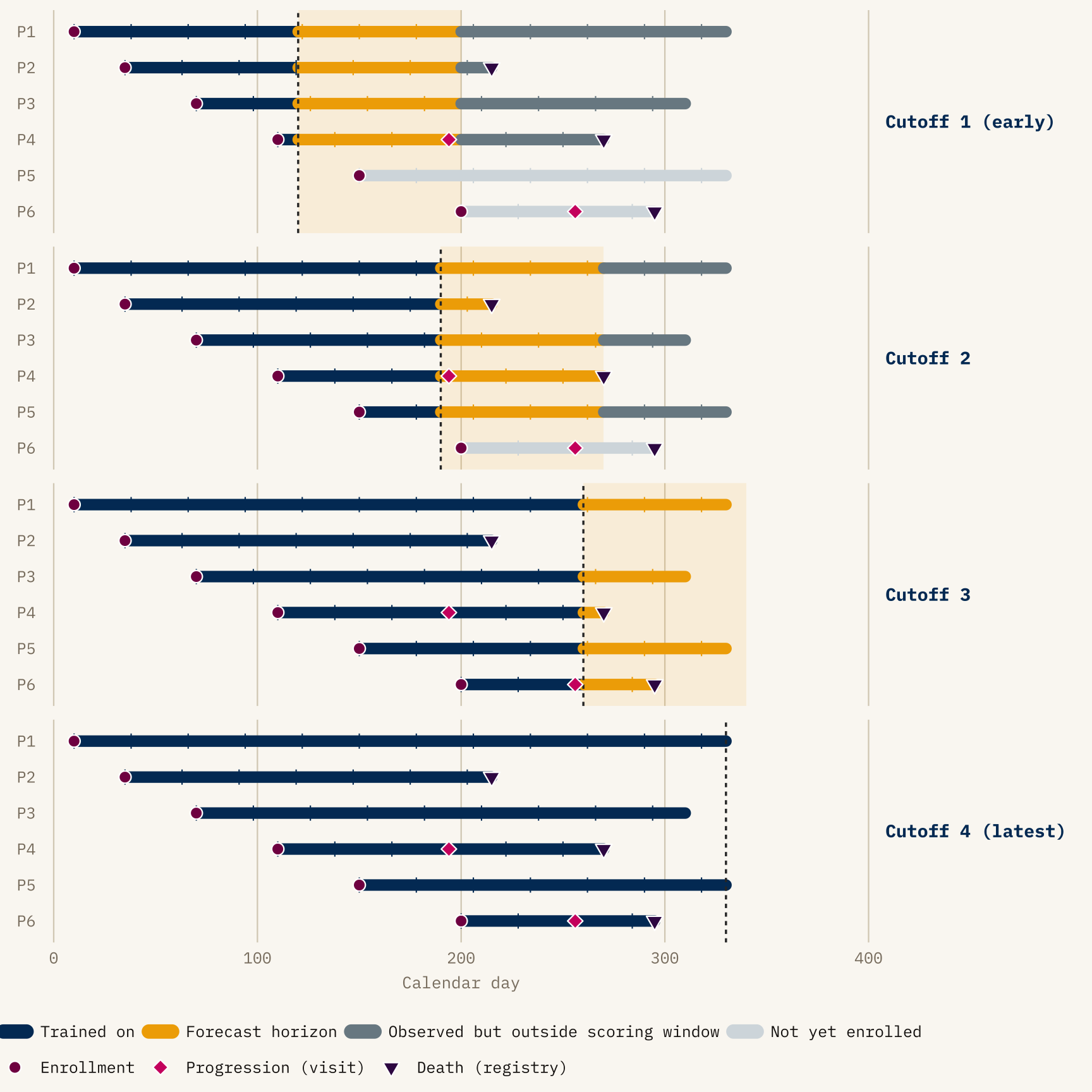
The diagram isolates three things that make LFO different from LOO on this kind of data.
- The training region grows with the cutoff — every panel refits on strictly more data, never less.
- Staggered enrollment interacts with the cutoff: a patient not yet in the trial at Cutoff 1 contributes nothing to that fold (greyed-out rail), and is evaluated only from later cutoffs onward.
- Events are categorized by which side of the cutoff they fall on — progression diamonds and death triangles in the navy region were known to the model, those in the gold band are what the model’s forecast is scored against, and anything beyond the gold band is outside the scoring horizon for that cutoff.
The split between progression (pink diamonds, observed only at clinic visits) and death (dark plum triangles, observed exactly from registry linkage) is deliberate: the rest of the post is largely about what happens when those two observation mechanisms disagree about where the cutoff lies.
This post is about what it took to bring LFO across that gap. It focuses on methodology rather than results from any particular program. The anonymized figures below are illustrative in shape, but scrubbed of trial, arm, or patient-identifying detail.
2 What this post is, and is not, claiming as new
Before going further it is worth being explicit about what came before, because the question “given data up to time \(t\), how well do we predict events after \(t\)?” has a long history in biostatistics under names other than LFO.
The single most important precedent is the dynamic-prediction-from-joint-models program initiated by Rizopoulos (2011). It is the structural ancestor of what I do here: condition on a patient’s longitudinal history through a landmark time, generate posterior predictions of subsequent event times from a fitted joint model, and score those predictions on the still-at-risk cohort. Rizopoulos’s framework uses time-dependent ROC/AUC and Brier scores rather than ELPD, and is implemented today in JMbayes2; the more recent super-learner extension by Rizopoulos and Taylor (2023) uses V-fold cross-validation over subjects with expected quadratic prediction error and predictive cross-entropy as scoring rules. None of this is LFO in the Bürkner et al. (2020) sense, but it is unambiguously the same question with different machinery.
Running parallel to that is the landmarking literature — the original landmark Cox model (van Houwelingen 2007), and the more recent “Landmarking 2.0” paper by Putter and van Houwelingen (2021), which deliberately reframes landmark analysis as a competitor to joint-model dynamic predictions. Landmarking already does, in spirit, exactly what LFO does: refit at a sequence of landmark times, evaluate prediction quality on data after each landmark. Devaux et al. (2022) take this further by combining landmarking with machine learning and cross-validated time-dependent Brier and AUC.
Against that backdrop, the contribution of the work in this post is narrower than “LFO for survival.” It is closer to:
- Porting the Bayesian ELPD-LFO machinery (Bürkner et al. 2020, plus the broader Vehtari
looecosystem) into a hierarchical joint longitudinal–multistate model in Stan, where the landmarking and AUC/Brier literatures already live; - Working out an observation-mechanism-aware re-censoring rule for that setting — specifically, the dual visit-week / calendar-week cutoffs — which the time-series LFO literature does not need and the joint-model dynamic-prediction literature has not, as far as I can find, written down explicitly;
- Wiring the whole thing into a pipeline that runs exact refits on a calendar-cutoff schedule and reports both decomposed ELPD and posterior-predictive Kaplan-Meier overlays per cutoff.
I do not claim novelty for the principle. I do claim usefulness for the specific construction, and I think the construction generalizes beyond the setting it was built for. The rest of the post is mostly about what the construction has to look like once you take the structure of oncology trial data seriously.
3 What LFO is, before we complicate it
The minimal (2020) LFO is easy to state. Let \(y_{1:T}\) be a univariate time series. For each candidate cutoff \(t_c\), fit the model on \(y_{1:t_c}\) and evaluate the expected log predictive density on what comes next:
\[ \text{ELPD}_{\text{LFO}} = \sum_{c} \sum_{t > t_c} \log p(y_t \mid y_{1:t_c}). \]
Two things make this useful. First, no future data leaks into training — the evaluation respects the causal structure of the data. Second, ELPD differences between models have a Bayesian interpretation and an estimable standard error, so “model A forecasts better than model B” becomes a quantitative, rather than rhetorical, claim.
For our setting we will need a slightly more general form. Patients are indexed by \(i\), and the data we have on each one — visits, events — is a multidimensional history rather than a scalar. So the inner sum is over \((i, t)\) pairs that fall after each cutoff, and the conditioning is on whatever has been observed for all patients up to the cutoff:
\[ \text{ELPD}_{\text{LFO}} = \sum_{c} \sum_{(i, t) \in \text{future}(c)} \log p\bigl(y_{i,t} \mid y_{1:c}\bigr), \]
where \(y_{1:c}\) is the cohort-level data up to cutoff \(c\) and \(\text{future}(c)\) is the set of patient–time pairs whose observations the model is being asked to forecast at \(c\). Picking \(\text{future}(c)\) correctly — which patients, which observation channel, up to which clock — is what most of the rest of the post is about.
The practical cost, of course, is refitting. A naive implementation requires one MCMC run per cutoff. Bürkner et al. (2020) show that for many models you can get away with a single full refit and then slide the cutoff using PSIS weights, triggering a refit only when the Pareto \(\hat k\) diagnostic signals that importance sampling has broken down. That trick is what makes LFO tractable in practice.
4 The joint model, briefly
The rest of the post discusses an LFO construction built around a particular model, so a quick sketch here will save backtracking.
The model has two coupled components, fitted jointly:
- A longitudinal state-space model for each patient’s tumor-burden trajectory — specifically, the sum of target-lesion diameters (SLD). Latent SLD trajectories are parameterized per patient (baseline, shrinkage, regrowth) with hierarchical pooling across the trial structure. SLD is observed only at scheduled imaging visits, and the target-lesion component of RECIST (CR / PR / SD / PD, driven only by SLD changes relative to baseline and nadir) is read off the SLD trajectory deterministically. Non-target response and new-lesion appearance are separate inputs to a full RECIST classification and sit outside this component.
- A three-state multistate hazard model for events: state 0 (on study, no recorded progression), state 1 (progressed), state 2 (dead). Three transitions are modelled — \(0\to 1\), \(0\to 2\), \(1\to 2\). The \(0\to 1\) transition has two sources: target-lesion progression, which is a deterministic function of the SLD trajectory once it crosses the RECIST threshold, and non-target/new-lesion progression, which is modelled probabilistically with its own hazard. Both can only be declared at a visit. The \(0\to 2\) and \(1\to 2\) transitions are modelled as standard survival hazards and are reported continuously through registry records.
The two components are coupled because the event hazards depend on the latent tumor state, not only on the SLD values that happen to be observed at visits. That dependence is what makes the model “joint” in the dynamic-prediction sense, and it gives the factorization
\[ p(\text{SLD}_i, \text{MS}_i \mid \theta) = p(\text{SLD}_i \mid \theta)\, p(\text{MS}_i \mid \text{SLD}_i, \theta), \]
where \(\theta\) collects all model parameters — the population-level trajectories, the per-patient random effects, and the multistate hazard coefficients.
which the ELPD decomposition later in the post rests on. Three things to carry forward: SLD lives on a visit clock, the multistate model lives on mixed clocks, and the hazards see the latent tumor state.
5 Where time series LFO breaks for oncology
Take a typical phase-II or phase-III oncology trial. Patients are enrolled continuously over eighteen months or so. Each patient has:
- a latent tumor burden trajectory, observed at irregular visits through sums of lesion diameters (SLD),
- a baseline covariate profile (prior lines of therapy, PD-L1 status, metastatic sites, …),
- a set of potential event times: target-lesion progressive disease (target PD), non-target progression, death,
- a cluster membership (trial, arm, potentially site),
- and, above all else, a calendar day of enrolment which is not the same as anyone else’s.
Any sensible predictive evaluation at a data cutoff \(D\) has to answer several uncomfortable questions at once:
Whose data counts? A patient enrolled after \(D\) has never been seen by the model; their trajectory is out-of-sample in a much stronger sense than a visit occurring after \(D\) for an already-enrolled patient. Are we evaluating the model’s ability to forecast existing patients’ futures, or its ability to generalize to unseen patients, or both? These are different tasks and they deserve different evaluations.
Which clock do we cut on? Tumor measurements are only made at visits. Deaths are observed exactly (to the day, typically from registry linkage). A patient whose last visit before the cutoff was week 14 but who dies at week 31 — where \(D\) falls after week 31 — has a known death that was never recorded at a visit. Cutting by visit would throw that information away. Cutting by calendar day alone would assume we observe progression continuously, which we do not.
What are we scoring? The primary model output might be a posterior-predictive Kaplan-Meier for overall survival. It might be a RECIST confusion matrix. It might be the joint log likelihood over the SLD stream and the multistate event stream. These are not interchangeable; they have different units, different sensitivities, and different clinical meanings.
None of these questions has a counterpart in the Bürkner et al. (2020) time-series LFO. They are not failures of the original method — they are features of the problem.
6 The shape of the solution
The rest of this post is about how my LFO implementation, built on top of the joint longitudinal–multistate model sketched in the previous section, handles each of those questions. I will not try to show all the code; the key pieces I point at are in a modular Stan include system and a small R pipeline of helper functions. The architecture matters less than the ideas behind it.
6.1 Calendar-day cutoffs on patient-specific clocks
The first design decision: cutoffs are calendar dates, not study weeks. A cutoff of 2025-09-30 translates, for each patient, into a different study week — specifically, the week of that patient’s last pre-cutoff visit on their own time axis. This is handled in Stan by a per-patient date arithmetic step: given the patient’s enrolment calendar day and the global cutoff, compute the patient’s cutoff in their internal week scale, then walk the patient’s visit array backwards to find the last visit that falls at or before it.
int patient_cutoff_study_day =
    calendar_date_to_study_date(patient_calendar_day[i], cutoff_calendar_day);
// ... find last visit day <= patient_cutoff_study_day, record its week.
This is the innocuous-looking conversion that makes everything else well-defined. Without it, a shared cutoff means very different things for a patient enrolled early in the trial (lots of follow-up) and a patient enrolled late (perhaps only one or two visits past baseline).
6.2 Two cutoffs per patient, for two observation mechanisms
At any calendar cutoff, what we know about a patient arrives through two separate channels:
- Imaging visits. Tumor size, RECIST category, and therefore target-lesion progression are measurable only at scheduled visits. Between visits, the tumor state is silent.
- Registry records. Deaths are reported to the exact day, continuously, from sources independent of the visit schedule.
These two channels do not run up to the same point on the patient’s timeline. At any calendar cutoff, visit information ends at the patient’s last pre-cutoff visit. Registry information ends at the calendar cutoff itself. A patient whose last visit was week 14 but who is known to have died at week 31 through a registry report has visit data that ends at week 14 and registry data that ends wherever the calendar cutoff falls — week 40, say. The same cutoff date produces two different “last-known” points on the same timeline.
Figure 2 shows what goes wrong if you try to collapse both into a single cutoff time. If you censor everything at the last visit, you throw away the week-31 death that the registry told you about. If you censor everything at the calendar cutoff, you implicitly insert phantom visits at weeks 21, 28, 35 that were never actually performed — meaning the patient would have to be classified as progression-free through those weeks on the basis of data that does not exist.
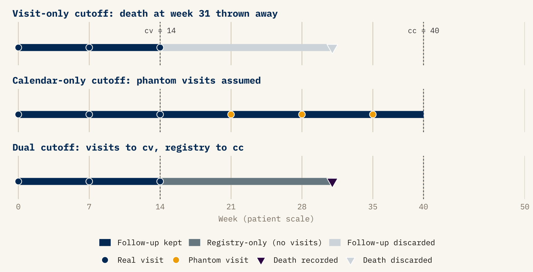
cv = cutoff_visit_week and cc = cutoff_cal_week. Top panel: censoring at cv alone discards the registry-recorded death (faded triangle) and treats the patient as alive-at-last-visit. Middle panel: censoring at cc alone implicitly inserts phantom visits (gold ticks) between week 14 and week 40 that the trial never observed. Bottom panel: the dual rule keeps visit-derived information up to cv and registry-derived information up to cc, so the death at week 31 is correctly attributed and no progression is fabricated.
The re-censoring rule is then just: use each channel up to its own “last-known” point, and nothing beyond.
- For anything visit-observed — progression, continued at-risk follow-up, RECIST category — take the patient up to the last pre-cutoff visit, and treat everything after that as unknown.
- For anything registry-observed — death, whether or not it followed a recorded progression — take the patient up to the calendar cutoff itself, and treat anything after it as not yet happened.
When an event crosses the cutoff, it is rolled back one step: a progression recorded after the last visit reverts to at-risk follow-up, a post-cutoff death reverts to whatever state the patient was in before dying. Patients not yet enrolled at the calendar cutoff have no visit history and no registry follow-up to keep; they are dropped from that cutoff’s evaluation entirely. This rule is packaged in a single Stan function, but the rule itself is the point, not the function.
I want to stress that this is not a technicality. It is the operational definition of what LFO means when applied to a multistate survival process where different transitions are observed through different mechanisms. Getting it wrong quietly inflates or deflates predictive accuracy depending on which direction the error pulls, and you will only catch it by checking that observed and posterior-predictive Kaplan-Meier curves at each cutoff match in the training region — a check worth automating into the pipeline and one I recommend anyone adapting this approach do the same.
6.3 Scoring: decomposed ELPD plus endpoint-level KM
With re-censoring settled, the rest of the evaluation is comparatively straightforward, but worth laying out for clarity.
The full log predictive density at a cutoff decomposes cleanly, along the same factorization as the model itself:
\[ \log p(y_i^{\text{future}} \mid y_i^{\text{past}}, \theta) = \underbrace{\log p(\text{SLD}_i^{\text{future}} \mid y_i^{\text{past}}, \theta)}_{\text{tumor component}} + \underbrace{\log p(\text{MS}_i^{\text{future}} \mid \text{SLD}_i, y_i^{\text{past}}, \theta)}_{\text{multistate component}}. \]
Summing over patients and cutoffs, and averaging over the posterior of \(\theta\) from each refit, gives a total ELPD and two sub-totals. The sub-totals are diagnostically valuable: a model that forecasts SLD well but multistate transitions poorly tells you something quite different from a model that fails symmetrically, and the decomposition makes which half is struggling immediately visible.
Alongside ELPD I track two endpoint-level diagnostics:
- Cutoff-by-cutoff Kaplan-Meier overlays. At each cutoff I plot the posterior-predictive KM (overall survival, PFS, per-arm or per-subgroup) from the refit at that cutoff, and let subsequent cutoffs’ observed curves fill in the region that was “future” at the time. This is where LFO earns its keep visually: a model that looks fine when the observed curve is averaged over the whole study can still be persistently too-optimistic between two adjacent cutoffs, and that is exactly the kind of miss no single summary number flags. Posterior-predictive vs observed KM at a fixed cutoff is a standard joint-model check; what is new here is that the comparison is made against later observed reality, not against the training cohort that produced the fit.
- RECIST confusion matrices aggregated over all out-of-sample visits and cutoffs, from which I compute per-class sensitivity and specificity. This is a side benefit of the joint model: once the tumor trajectory is forecast, the RECIST classification is deterministic, so “how often did the model correctly predict that this patient would be in progressive disease a year from the cutoff?” becomes a quantity with a posterior distribution.
6.4 Exact refits vs PSIS: when is the shortcut safe?
The Bürkner et al. (2020) PSIS-LFO trick is tempting, and the pipeline supports it (max_n_rows = n_cutoffs with a forecast horizon spanning all cutoffs, triggering a single refit whose posterior is reweighted at each cutoff). In practice, I default to exact refits. The reason is specific to the problem: when the cutoff moves, the structure of the data changes, not just its volume. A patient who was at-risk at cutoff \(c_1\) may be in state 1 at cutoff \(c_2\); a patient enrolled between \(c_1\) and \(c_2\) is admitted to the likelihood only at the later cutoff. The mapping from posterior at \(c_1\) to the likelihood at \(c_2\) is therefore not the simple “add a few more observations” that PSIS handles gracefully. The Pareto \(\hat k\) diagnostic flags this reliably, but by the time you have diagnosed it across several cutoffs you have effectively paid the cost of refitting anyway. For production evaluation I run exact refits on a schedule of cutoffs spaced by a configurable number of days, starting at the first landmark-eligible date. For development iteration, PSIS is a useful shortcut.
6.5 Standard errors: why the time-series recipe does not transfer
In the Bürkner et al. (2020) setting, uncertainty in the ELPD estimate comes from a single analytic formula: if the \(T\) pointwise log scores are treated as exchangeable contributions, then the SE is \(\sqrt{T \cdot \widehat{\mathrm{Var}}_t(\hat\ell_t)}\). That is what loo reports, and it works because the summation unit — time \(t\) on a single series — is also the unit the exchangeability assumption is pinned to.
In the oncology setting that assumption fails twice over. A single patient contributes correlated scores across their own visits, and the same patient reappears at every cutoff they were enrolled for. So the \((i, t, c)\) contributions inside the ELPD sum are heavily nested: not \(T\) independent draws, but rather \(\sim N\) patient-clusters, each contributing many correlated scores. Treating them as independent — which is what the time-series formula does — counts the same evidence many times over and produces an SE that dramatically understates uncertainty.
We therefore need an SE estimator built around the right unit of independence. Across patients we are willing to assume exchangeability (that is exactly the assumption the hierarchical model encodes); within a patient we are not. The natural way to express that asymmetry without a closed-form variance derivation is a non-parametric bootstrap over patients: simulate the variability we would see if we had drawn a different cohort of patients from the same population, and let the empirical spread of ELPD across simulated cohorts stand in for the SE.
Concretely: at each bootstrap replicate I draw \(N\) patient indices with replacement from the trial cohort. For those patients (and only those), I re-evaluate the ELPD — summing each patient’s contribution across the visits and cutoffs at which they were observed — and record a single number \(\text{ELPD}^{(b)}\). Repeating \(B\) times gives a distribution of ELPD estimates over hypothetical cohorts, and the standard deviation of that distribution is the reported SE.
There is one subtlety in the re-evaluation step, and it is where PSIS comes back in. At cutoff \(c\) my exact refit gives posterior draws from \(p(\theta \mid y_{1:c})\) — conditional on the full cohort at \(c\). But the replicate’s ELPD should really be evaluated under \(p(\theta \mid y^{(b)}_{1:c})\), the posterior I would have obtained had I trained on the bootstrapped patients only. Refitting per replicate is hopelessly expensive, so I use the same importance-reweighting trick PSIS uses in ordinary LOO: reweight the full-cohort posterior draws by the ratio of bootstrap-subsample likelihood to full-cohort likelihood, smooth the weights with Pareto \(\hat k\), and compute the replicate’s per-patient scores against the reweighted draws. The move is mathematically the same as LOO’s \(p(\theta \mid y_{-i}) \approx\) reweighted draws from \(p(\theta \mid y)\), just with a different target posterior: “condition on the bootstrap subcohort” instead of “condition on everything except \(i\).” The weights are recomputed fresh for every replicate × cutoff combination, so the importance-sampling correction always matches the cohort being scored.
Two things to notice about this construction. First, because each replicate carries a whole patient with all of their visits and all of their cutoff appearances bundled into one draw, the within-patient correlation that broke the analytic formula is absorbed automatically: a patient is in or out of replicate \(b\) as a unit, never as a collection of pseudo-independent rows. Second, the SE is interpreted as cohort-resampling uncertainty, not posterior uncertainty in \(\theta\) — the latter is already folded into each \(\hat\ell_{i,c}\) when we average over posterior draws. The bootstrap is doing the work the analytic formula was trying to do (estimate cohort-level sampling variability), with an exchangeability assumption we are actually willing to make.
Two caveats are worth flagging rather than hiding.
The first is that PSIS now plays two roles — the between-cutoff approximation from the previous section, and the within-replicate reweighting just described — and a \(\hat k\) failure in either one matters. The bootstrap drops cutoffs that fail the reliability filter at either stage, so the reported SE is conditional on PSIS-reliable cutoffs and bootstrap subcohorts. If the dropped configurations are systematically the most uncertain ones, the SE under-covers. When \(\hat k\) degrades for the within-replicate reweighting specifically, the honest fix is to reduce the effective step size of the bootstrap (resample fewer patients out at a time, e.g. via blocked resampling) or, in the limit, refit per replicate — the latter is rarely tractable, but the former is on the to-do list.
The second is more consequential and worth stating plainly: my current implementation resamples patients independently per model. That gives correct marginal SEs for each model’s absolute ELPD, but it is wrong for model comparisons. The variance identity
\[ \mathrm{Var}(\text{ELPD}_A - \text{ELPD}_B) = \mathrm{Var}(\text{ELPD}_A) + \mathrm{Var}(\text{ELPD}_B) - 2\,\mathrm{Cov}(\text{ELPD}_A, \text{ELPD}_B) \]
requires a covariance that an unpaired bootstrap cannot identify. Two models scored on the same patients tend to produce highly positively correlated per-patient ELPDs — if patient \(i\) is an outlier, both models will struggle with them — and the correct paired-bootstrap SE of the difference is typically much smaller than \(\sqrt{\mathrm{Var}(A) + \mathrm{Var}(B)}\). This is exactly why loo_compare reports a paired SE on ELPD differences rather than the individual model SEs in quadrature. In my current setup, the two models’ bootstrap replicates come from independently drawn patient index sets, so differences of replicates do not estimate \(\mathrm{Var}(A - B)\) — they estimate \(\mathrm{Var}(A) + \mathrm{Var}(B)\), which is inflated.
The bias is one-sided: unpaired SEs of differences are conservative, so I have probably been understating the confidence with which one model out-forecasts another, not overstating it. Still, the fix is mechanical (draw one set of patient indices per replicate and apply it to all models) and is next on the list of pipeline corrections. Anyone adopting a patient-level bootstrap for multi-model LFO comparisons should plan for this from the start: the exchangeable unit you resample needs to be held constant across the models you compare.
7 Why this matters more broadly
I want to pull back from the specifics and say something about the broader case.
For Bayesian modelers familiar with loo and LFO from the time-series side. The temporal-integrity principle underlying LFO generalizes beyond univariate series, but generalizing it requires explicit design choices about (a) who is in the evaluation cohort at each cutoff, (b) which clock each observation uses, and (c) what quantity you are scoring. These choices are not downstream implementation details; they determine what the ELPD number actually means. The single piece of the implementation I would single out as worth borrowing is the dual-cutoff re-censoring — it is the place where the biostatistical reality of the data leaks into the Bayesian formalism, and as far as I can find it does not appear in the existing LFO literature.
For oncology biostatisticians familiar with landmarking and joint models. Most of what LFO buys you here is already available in your toolkit, just under different names. Landmarking and dynamic prediction from joint models (Rizopoulos 2011; van Houwelingen 2007; Putter and van Houwelingen 2021) ask the same temporal question. What ELPD-LFO adds is (i) a single coherent log-predictive scoring rule that decomposes cleanly into longitudinal and event components for joint models, and (ii) a Bayesian posterior over the score itself, with estimable standard errors for model comparison. Whether you want that on top of time-dependent AUC and Brier scores is a real question; my own view is that they are complementary, not substitutes, and that ELPD-LFO is most useful when comparing competing generative mechanisms rather than competing point predictions. Practically, the cutoff-by-cutoff KM overlay is the diagnostic that has earned its keep most reliably in conversations with stakeholders.
For people working in other domains entirely. The structure of the problem — multiple actors entering the system at different times, a latent mechanistic process generating both longitudinal and event streams, different observation mechanisms for different outcomes — is not unique to oncology. Infectious-disease surveillance with serology and case reports, reliability engineering with sensor readings and failure events, and customer-lifetime modeling with usage logs and churn events all share the same skeleton. I suspect the pattern of calendar-cutoff LFO with observation-mechanism-aware re-censoring is directly portable, and I would be interested to hear from anyone who has tried it in a different context.
8 A short closing thought
There is a tendency, when importing a method from one literature to another, to keep it at the level of the name — “we used leave-future-out cross-validation” — without examining whether the assumptions the method was built on still hold. My experience with LFO in oncology has been that the principle transfers cleanly and is even more valuable here than in univariate time series, but that the machinery has to be rebuilt around the structure of the data: staggered enrolment, mixed observation clocks, competing risks, hierarchical pooling, and joint longitudinal–event likelihoods.
The pay-off for doing that work, at least for me, is that the ELPD numbers and KM overlays coming out of the pipeline feel trustworthy in a way that no in-sample criterion ever did. When a sponsor asks “how well will this model forecast?” I can point at a specific data cutoff from six months ago, show the forecast the model would have produced at that cutoff, and show where the observed curve landed. That is a conversation LFO makes possible, and one that internal goodness-of-fit cannot.
References
Andersen, Per Kragh, and Niels Keiding. 2002. “Multi-State Models for Event History Analysis.” Statistical Methods in Medical Research 11 (2): 91–115. https://doi.org/10.1191/0962280202SM276ra.
Andrinopoulou, Eleni-Rosalina, and Dimitris Rizopoulos. 2016. “Bayesian Shrinkage Approach for a Joint Model of Longitudinal and Survival Outcomes Assuming Different Association Structures.” Statistics in Medicine 35 (26): 4813–23. https://doi.org/10.1002/sim.7027.
Bürkner, Paul-Christian, Jonah Gabry, and Aki Vehtari. 2020. “Approximate Leave-Future-Out Cross-Validation for Bayesian Time Series Models.” Journal of Statistical Computation and Simulation 90 (14): 2499–523. https://doi.org/10.1080/00949655.2020.1783262.
Bürkner, Paul-Christian, Jonah Gabry, and Aki Vehtari. 2024. “Approximate Leave-Future-Out Cross-Validation for Bayesian Time Series Models.” https://mc-stan.org/loo/articles/loo2-lfo.html.
Cooper, Andrew, Daniel Simpson, Lauren Kennedy, Catherine Forbes, and Aki Vehtari. 2023. Cross-Validation Methods for ARX(p,q) Models.
Devaux, Anthony, Robin Genuer, Karine Pérès, and Cécile Proust-Lima. 2022. Individual Dynamic Prediction of Clinical Endpoint from Large Dimensional Longitudinal Biomarker History: A Landmark Approach.
Eisenhauer, E. A., P. Therasse, J. Bogaerts, et al. 2009. “New Response Evaluation Criteria in Solid Tumours: Revised RECIST Guideline (Version 1.1).” European Journal of Cancer 45 (2): 228–47. https://doi.org/10.1016/j.ejca.2008.10.026.
Gerds, Thomas A., and Martin Schumacher. 2006. “Consistent Estimation of the Expected Brier Score in General Survival Models with Right-Censored Event Times.” Biometrical Journal 48 (6): 1029–40. https://doi.org/10.1002/bimj.200610301.
Gneiting, Tilmann, and Adrian E. Raftery. 2007. “Strictly Proper Scoring Rules, Prediction, and Estimation.” Journal of the American Statistical Association 102 (477): 359–78. https://doi.org/10.1198/016214506000001437.
Houwelingen, Hans C. van. 2007. “Dynamic Prediction by Landmarking in Event History Analysis.” Scandinavian Journal of Statistics 34 (1): 70–85. https://doi.org/10.1111/j.1467-9469.2006.00529.x.
Putter, Hein, and Hans C. van Houwelingen. 2021. Landmarking 2.0: Bridging the Gap Between Joint Models and Landmarking.
Rizopoulos, Dimitris. 2011. “Dynamic Predictions and Prospective Accuracy in Joint Models for Longitudinal and Time-to-Event Data.” Biometrics 67 (3): 819–29. https://doi.org/10.1111/j.1541-0420.2010.01546.x.
Rizopoulos, Dimitris, and Jeremy M. G. Taylor. 2023. Optimizing Dynamic Predictions from Joint Models Using Super Learning.
Vehtari, Aki. 2024. “Cross-Validation FAQ.” https://avehtari.github.io/modelselection/CV-FAQ.html.
Vehtari, Aki, Andrew Gelman, and Jonah Gabry. 2017. “Practical Bayesian Model Evaluation Using Leave-One-Out Cross-Validation and WAIC.” Statistics and Computing 27 (5): 1413–32. https://doi.org/10.1007/s11222-016-9696-4.
Footnotes
RECIST (Response Evaluation Criteria in Solid Tumors) is the standard classification scheme used to summarize tumor response in oncology trials. Each patient visit is assigned one of four categories — complete response (CR), partial response (PR), stable disease (SD), or progressive disease (PD) — based on changes in the sum of target-lesion diameters relative to baseline and the nadir, together with the appearance or progression of non-target lesions. The current version is RECIST 1.1 (Eisenhauer et al. 2009). For the purposes of this post, the relevant facts are that RECIST categories are (i) observable only at imaging visits, not continuously, and (ii) the target-lesion component of the classification is a deterministic function of the underlying tumor-size trajectory — which is the part this post’s model handles.↩︎